Estimating your probabilities Understanding logistic regressions

By tossing a coin once, what is the probability of having a head? Easy question. If a coin is fair, it is 50%. In other words, if you bet a head as outcome and it realized, you succeed. If not, you failed. Succeed or not succeed, occurrence or not occurrence, gain a sale or do not gain, all these outcomes can be translated as 0 and 1. The coin is one of the cases where you cannot control the probabilities. However, in the real world, the events do not occur randomly, without any control of the outcomes, and for us, it is just a matter of proper identifying the variables that affect these probabilities. Concretizing a sale may be achieved by adjusting the product price, improving quality and advertising spending, etc. Employee attrition may be controlled by identifying the most effective incentives and avoiding those that, in this case, are positively correlated to the employee attrition. And so on. In this article I will show you one technique used to identify and estimate these probabilities: the logistic model. By using this model, you can also identify the variables that most impact the results. But before some concepts. You may skip the next topic, if you desire, going directly to the topic 2 and 3.

1. Some concepts

Succeed / not succeed is a binary outcome that follows what is called Bernoulli distribution with p probability to occur and 1-p probability to not occur, and the sum of p and 1-p is 1 (100%).

The Bernoulli distribution is a special case of the binomial distribution where a single trial is conducted (so n would be 1 for such a binomial distribution) and sometimes is written as:

Since the response is a binary variable, many data scientists use linear regression to estimate these probabilities (0 and 1). Is this a good practice? Actually, is not adequate to use linear model in this case. Consider the following linear equation:

If Ŷi is a binary response (0 or 1) the adjusted regression should be:

The above equation represents the linear probability model (LPM) and correspond to a straight line. In this case, no one can guarantee the outcomes (Pi or Yi) will respect the boundaries [0,1]. Depending on the Xi value Ŷi might be negative or higher than 1 unless the following restrictions are applied:

1 – if Ŷi is negative then consider 0 as prediction

2 – if Ŷi is higher than 1 then consider 1 as prediction

Below the figures representing the LPM without (a) and with constraints (b):

A better way to properly guarantee that the estimated conditional probabilities E(Yi) will lie between 0 and 1 is using probit or logit models. Both have similar results but, in this article, I will show how to extract useful information from the logit model (or logistic regression model). Differently from the linear model, where the probability is a linear transformation of the variable Xi (Pi = β1 + β2Xi), in a logistic regression model the probabilities of occurrence and non-occurrence are given by:

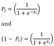
where the term zi = β1 + β2Xi and is called logit.

Note in the figure below that the logit is a linear transformation of X and the probability function turns to a sigmoid curve from -inf to + inf with the boundaries [0,1].

An interesting metric is called odd ratio: p/(1-p). It represents how much the probability of occurrence is higher (or lower) than non-occurrence. So, for example, if the probability of sales occurrence is 0.8, the non-occurrence is 0.2. In this case, the odd ratio is 4, indicating the probability of occurrence is 4x higher than non-occurrence. A 50/50 chance (like our coin) has an odd ratio of 1. So, if the occurrence is a good event (like sales) the best action is to keep this ratio above 1, and the probability of sales will be higher than the probability of non-sales. Conceptually, the logit is calculated from this metric as the logarithm of the odd ratio (the probability of occurrence divided by non-occurrence).

In addition, if:

 2. Why does all this stuff matter?

The analysis is quite simple. If the logit represents the logarithmic of the odd ratio, we can find how much the variable X will impact an event occurrence, just by finding the exponential of the coefficients (remember: the exponential is also called anti-log).

For better visualization, consider the hypothetical example. Suppose you have a large database with historical inquiries from your customers with some inquiries where the customer confirmed the sales order (1) and some inquiries where the customer did not confirm (0). In this situation, half of the customers purchased your products and half did not, so your current odd ratio is then, 1 (50%/50%).

You know you are not competing in a market with homogeneous products (when customers don’t perceive differences between your products and the products from your competitors), so in this case you must identify from the database the relevant variables that would lead customers to firm the orders in addition to the product price. Since your products have some degree of differentiation, variables like product durability, guarantee, price, product capacity and speed (supposing a laptop) and many other ‘qualities’ perceived by the customers must be added to the model. You did that and after executing a logistic regression, you found the following equation:

Sales (yes or no) = -25.93 + 0.3(guarantee) + 0.5(durability) - 0.10(price)

To short this exemplification, let’s suppose the other variables were not statistically significant, only these 3. Guarantee is measured in months, durability measured in years and price measured in 000/USD. Question: What do the coefficients tell you about the probability of sales?

Guarantee: the coefficient is 0.3 so, keeping all the other predictors constant, the probability of a customer firming the order increases by 0.3*(0.5*0.5) = 7.5% to each month added in guarantee. The previous probability will increase from 50% to 57.5%, and the odd ratio will increase 35% (0.575/0.425 = 1.35). This increase in odd ratio is confirmed by exponentializing the coefficient:

Durability: the coefficient is 0.5 so, keeping all the other predictors constant, the probability of a customer firming the order increases by 0.5*(0.5*0.5) = 12.5% to each year added to durability. The previous probability will increase from 50% to 62.5%, and the odd ratio will increase 66% (0.625/0.375 = 1.66). This increase in odd ratio is confirmed by exponentializing the coefficient:

Price: in this case the coefficient is negative (-.10) so, keeping all the other predictors constant, the probability of a customer firming the order decreases by -0.1*(0.5*0.5) = -2.5% to thousand dollars added to the product price. The previous probability will decrease from 50% to 47.5%, and the odd ratio will decrease 10% (0.475/0.525 = 0.90). This decrease in odd ratio is confirmed by exponentializing the coefficient:

Notice that this is a cold analysis with hypothetical numbers, just for contextualize how powerful is the logistic regression. In our example, improvement in quality may cause a price increase and the results in sales would be a net percentual considering increases in durability and price. Another point: improvement in durability might also jeopardize your own demand (product last longer), so instead of a good result you may have the opposite (a decrease in the number of orders placed by your customers).

3. Other examples of the model application

There are many other examples of the usage of this technique, here’s some:

• Credit risk analysis based on customer income, past defaults, current debt amount, etc.

• Employee attrition based on job satisfaction, monthly income, overtime, home distance, etc.

• Customer approval based on product characteristics, as for example, wine quality based on the physicochemical characteristics (Wine Quality - UCI Machine Learning Repository). In this case the response variable ranges from 1-10, so it is not binomial. Someone may consider lower than 7 as a bad taste and higher or equal to 7 as a good taste. Another option is using multinomial logistic regression. But it is a topic for another article…